Performance

magpylib_jax is built for repeated evaluations and differentiable outer loops. This page has two halves: how to make your own code fast (JIT, vmap, accelerators, honest timing), and how the library measures itself (benchmarks and the profiling pipeline).

Repeated eager calls are cached automatically

Calling src.getB(obs) (or magpy.getB("cuboid", obs, …)) in a loop no longer re-does the Python-side source/observer preparation every time. The first call for a given (source type, array shapes) compiles a jitted evaluation with the parameters and pose passed as traced arguments; every later call — including a loop that changes the geometry or excitation each step — reuses the compiled function without re-tracing. On CPU a single Cuboid over 10 000 observers dropped from ~124 ms to ~1.5 ms per call (~80×), and a three-source Collection from ~117 ms to ~4.8 ms (~24×). Gradients are unaffected: under jax.grad/jit the cache is bypassed and the computation traces as usual. See scripts/profile_workloads.py to measure it on your machine.

Note

The Cylinder (elliptic-integral) and CylinderSegment (surface-mesh) kernels are the heaviest per observer; the latter trades the full analytic tile formula for a differentiable surface mesh, so it is the slowest source. For very large sweeps prefer batching over observers (below) and keep them on a GPU/TPU.

Make your code fast

JIT your function, not just the field

The public getB/getH/getJ/getM path already runs through a JIT-safe core, but the big wins come from compiling your whole computation — loss, field, and reduction together — so XLA can fuse it and you pay the tracing cost only once.

import jax
import jax.numpy as jnp
import magpylib_jax as mpj

obs = jnp.array([[0.2, 0.1, 0.4], [0.5, 0.0, 0.7]])

@jax.jit
def loss(pol):
    B = mpj.magnet.Cuboid(dimension=(1.0, 0.8, 1.2), polarization=pol).getB(obs)
    return jnp.sum(B ** 2)

grad = jax.jit(jax.grad(loss))     # compiled forward + backward pass

Keep shapes static

JAX recompiles when array shapes change. Keep your observer layout, pixel grid, and number of sources fixed across iterations so a compiled function is reused instead of re-traced.

Batch with vmap

To sweep a parameter — many polarizations, many geometries, many observer clouds — write the single-case function once and map it. No Python loop, and the batch compiles to one fused kernel:

import jax
import jax.numpy as jnp
import magpylib_jax as mpj

OBS = jnp.array([[0.2, 0.1, 0.4], [0.5, 0.0, 0.7], [-0.3, 0.2, 0.5]])

def field(pol):
    return mpj.magnet.Cuboid(dimension=(1.0, 0.8, 1.2), polarization=pol).getB(OBS)

pols = jax.random.normal(jax.random.PRNGKey(0), (256, 3)) * 0.5
batched = jax.jit(jax.vmap(field))
out = batched(pols)     # shape (256, 3, 3): 256 sources x 3 observers x 3 components

Full script: examples/differentiable/jit_vmap_batching.py, and the walkthrough in Performance examples.

GPU and TPU

The field core is plain JAX/XLA, so the same code runs on GPU and TPU with no changes — install the accelerator jax/jaxlib build for your platform and JAX places arrays on the device automatically. Accelerators shine on large batched workloads (big vmap sweeps, dense observer grids); for a handful of points on a small source, host-side preparation can dominate and CPU may be faster.

Time it honestly

JAX is asynchronous: an operation returns a future immediately and only blocks when you read the result. Two rules give trustworthy numbers:

1. Never time the first call — it includes tracing and compilation. Warm up once, then measure.

2. Call block_until_ready so you time the compute, not just the dispatch.

import time, jax

warm = jax.block_until_ready(batched(pols))     # compile + warm up (not timed)

t0 = time.perf_counter()
for _ in range(20):
    out = jax.block_until_ready(batched(pols))
per_call_ms = (time.perf_counter() - t0) / 20 * 1e3

The honest CPU benchmark

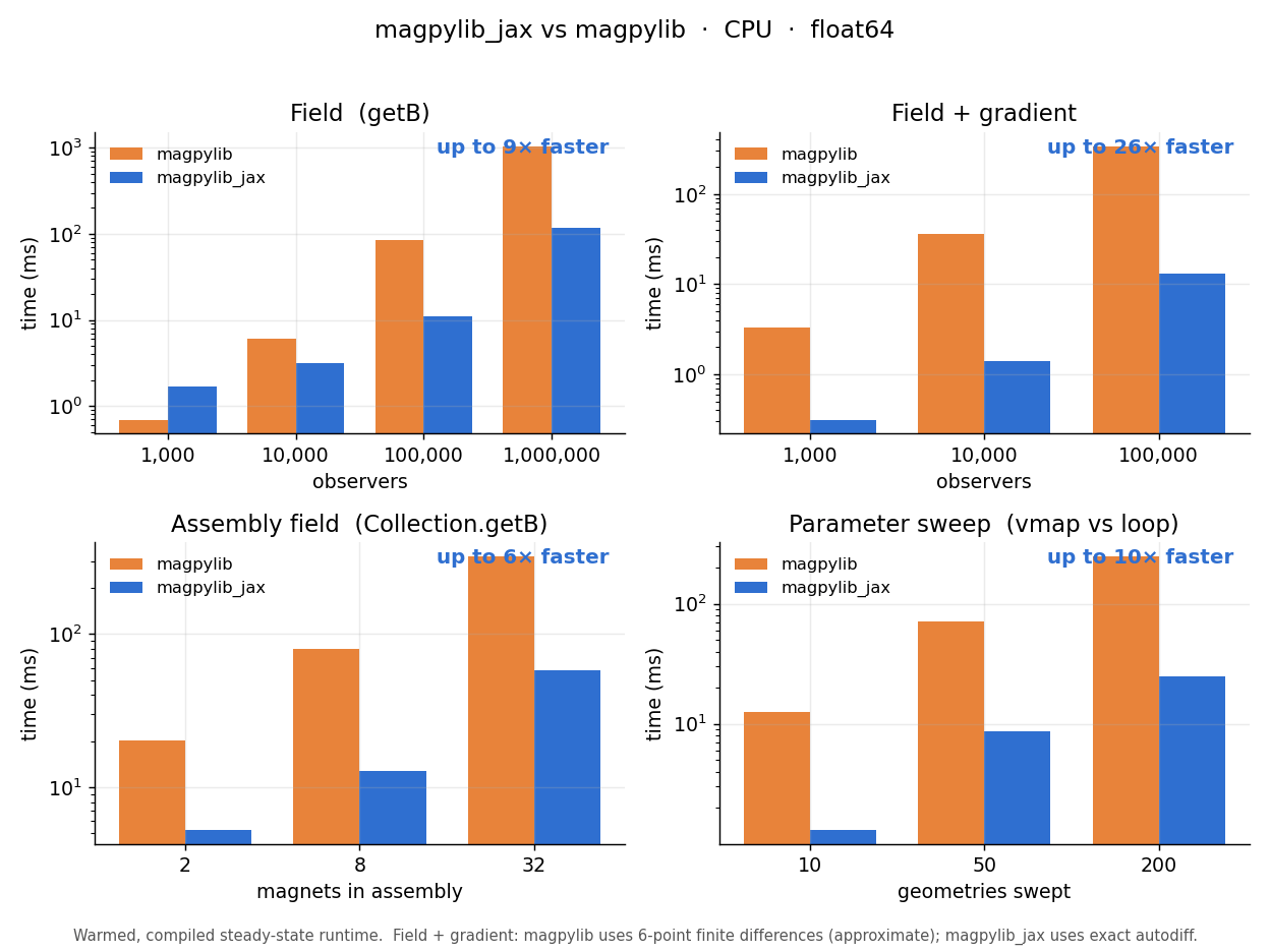
The figure above compares steady-state CPU runtime across four representative workloads — batched getB, field + gradient, a magnet Collection, and a vmap parameter sweep — against upstream Magpylib. Read it with the async caveats in mind: it reports compiled, warmed-up runtime, so it excludes JAX’s one-time compilation cost. The takeaways are practical rather than triumphal:

• After compilation the analytic kernels are competitive on CPU and pull ahead as work is batched (observers, assembly size, sweep width). Magpylib’s low-overhead NumPy still wins the smallest problems — visible in the leftmost bars.

• The field + gradient panel is the decisive one: Magpylib has no autodiff and must finite- difference (approximate, step-size dependent), while magpylib_jax returns the exact gradient in a single reverse pass.

• The first call to any new shape pays a compile cost — amortize it across an optimization loop.

• The real advantage is not raw CPU speed but that the same call is differentiable, vectorizable, and portable to GPU/TPU. Converting the JAX result back to NumPy has a cost too, and the benchmark scripts record it.

Regenerate the four-panel figure with scripts/make_benchmark_plots.py, and the per-source-family view (benchmark.png) with scripts/make_figures.py.

Reproduce on GPU / TPU

scripts/benchmark_gpu.py is a self-contained micro-benchmark (needs only magpylib-jax) that prints a device-aware table of forward getB and field-plus-gradient timings. Run it on whatever backend JAX picks up — the report names the active device, so a run on a GPU/TPU host self-documents. In Google Colab with a GPU runtime:

pip install -q magpylib-jax
wget -q https://raw.githubusercontent.com/uwplasma/magpylib_jax/main/scripts/benchmark_gpu.py
python benchmark_gpu.py            # add --x64 for float64

Note

The published figures are measured on CPU. On a GPU the batched, fused kernels parallelize much further; drop the numbers from benchmark_gpu.py into a PR if you would like them added here.

Under the hood: high-level optimizations

The JIT-safe getB path avoids redundant host-side work through caching:

• source preparation caches keyed by object cache tokens,

• sensor preparation caches keyed by identity, path, pixel layout, and handedness,

• cached orientation matrices on the object base,

• cached Collection flatten/source/sensor lists with dirty propagation,

• reused TriangularMesh oriented faces and CylinderSegment face geometry,

• fast paths for circle-heavy collections and tiny observer batches.

A fast kernel can still yield a slow getB if this preparation dominates, which is why both layers are profiled.

Profiling pipeline

The repository profiles kernels and the high-level path separately and gates on the results.

Script	Purpose
profile_kernels.py	Per-family compile time, runtime, memory, HLO.
profile_getB_jit.py	High-level getB overhead.
profile_wham_workload.py	A representative double-coil workload vs. upstream.
check_profiling_thresholds.py	Enforce compile/runtime/memory thresholds.
check_hlo_diffs.py	Track HLO structure (report-only).

Each family run produces a JAX trace (jax.profiler.trace), an HLO dump (compiler_ir(..., dialect="hlo")), and a device-memory snapshot (jax.profiler.save_device_memory_profile).

What is gated, and what is not

Hard CI gates are parity error, compile/runtime thresholds, memory thresholds, benchmark thresholds, and the test/docs builds. Exact HLO hashes are useful for trend tracking but are intentionally report-only: unpinned JAX/XLA versions can restructure compiler output without changing correctness.

Threshold files:

• benchmarks/thresholds.json

• profiling/thresholds.json

• profiling/thresholds_getB_jit.json

Fixed-observer-count JIT entrypoints

For specialized high-throughput workloads with a fixed observer count and a single source family, core/kernels/ exposes wrappers that cache compilation by observer count (current_circle_bfield_jit, current_polyline_bfield_jit, triangle_bfield_jit, tetrahedron_bfield_jit, magnet_cylinder_segment_bfield_jit, …). These exist mainly for profiling and isolating compile/runtime behavior — for everyday use, the high-level getB path is the right default.

Workflow after a kernel change

1. Run profile_kernels.py; inspect compile/runtime/memory deltas.

2. Run profile_getB_jit.py if the change can touch the high-level path.

3. Compare parity outputs.

4. Update thresholds only when the change is intentional and justified.

5. Keep HLO baselines as observability aids, not the sole regression signal.