Force and torque (getFT)
mpj.getFT(sources, targets) returns the magnetic force F (N) and torque T (N·m)
that one or more sources exert on one or more targets. Unlike Magpylib, the magnet gradient is
taken with automatic differentiation, so the result is exact and carries no finite-difference
step size. The underlying physics is derived in
Equation Models — Force and torque.
Note
Run these examples with x64 enabled (jax.config.update("jax_enable_x64", True)) for
magpylib-grade accuracy.
Magnet in the field of a current loop
A cuboid magnet sits above a circular coil. getFT gives the force and torque the coil exerts on
the magnet.
import jax
import jax.numpy as jnp
import magpylib_jax as mpj

jax.config.update("jax_enable_x64", True)

coil = mpj.current.Circle(current=100.0, diameter=0.02)
magnet = mpj.magnet.Cuboid(
    dimension=(0.005, 0.005, 0.005),
    polarization=(0.0, 0.0, 1.2),
    position=(0.0, 0.0, 0.01),
)

F, T = mpj.getFT(coil, magnet)
print("force  (N):  ", F)
print("torque (N.m):", T)
F and T have shape (3,) here because there is a single source, a single path point, and a
single target (length-1 axes are removed when squeeze=True, the default). Pass squeeze=False
to keep the full (s, p, t, 3) layout used for batched sources, paths, and targets.
Autodiff gradient versus finite differences
For a magnet, the force is the gradient of the interaction energy,
Magpylib evaluates \(\nabla(\mathbf{m}\cdot\mathbf{B})\) with a finite-difference stencil controlled by
an eps step size. magpylib_jax evaluates the same gradient with jax.jacfwd, so it is exact and
independent of eps. The eps argument is still accepted for API compatibility but does not change
the result:
F1, _ = mpj.getFT(coil, magnet, eps=1e-3)
F2, _ = mpj.getFT(coil, magnet, eps=1e-7)
# identical: the autodiff gradient does not depend on eps
assert jnp.allclose(F1, F2)
Because the whole computation is differentiable, you can also differentiate the force itself, for example to obtain the force gradient (stiffness) along the vertical axis:
def fz(z):
    m = mpj.magnet.Cuboid(
        dimension=(0.005, 0.005, 0.005),
        polarization=(0.0, 0.0, 1.2),
        position=(0.0, 0.0, z),
    )
    F, _ = mpj.getFT(coil, m)
    return F[2]

stiffness = jax.grad(fz)(0.01)  # dF_z/dz  (N/m)
Dipole–dipole force
Point dipoles are the simplest targets. Here two moments are aligned along z and separated along
z; the force is attractive (points along -z on the upper dipole).
source = mpj.misc.Dipole(moment=(0.0, 0.0, 1.0))
target = mpj.misc.Dipole(moment=(0.0, 0.0, 1.0), position=(0.0, 0.0, 0.05))

F, T = mpj.getFT(source, target)
print("dipole-dipole force (N):", F)  # dominant component along z
Target meshing
Extended targets are discretized into cells before the per-cell force is summed. The discretization
is controlled by the target’s meshing attribute:
Cuboid— a grid of cells;meshingis aninttarget cell count or a(n1, n2, n3)tuple (default: a single cell).Circle— a polygon withmeshingsegments (default 100; minimum 3).Polyline—meshingpoints per segment (default 1).
Dipole and Sphere are single-cell targets and ignore meshing.
# refine the magnet target into an 8 x 8 x 8 grid of cells
fine_magnet = mpj.magnet.Cuboid(
    dimension=(0.005, 0.005, 0.005),
    polarization=(0.0, 0.0, 1.2),
    position=(0.0, 0.0, 0.01),
    meshing=(8, 8, 8),
)
F_fine, T_fine = mpj.getFT(coil, fine_magnet)
Finer meshing converges toward the continuum force at the cost of more field evaluations; a single cell is often enough when the target is small compared with the field’s spatial variation.
The pivot argument
The torque’s lever-arm term \(\mathbf{r}\times\mathbf{F}\) is taken about the pivot point:
pivot="centroid"(default) — each target’s own centroid (falling back to its position).pivot=None— omit the lever-arm term and return only the intrinsic torque \(\mathbf{m}\times\mathbf{B}\).pivot=(x, y, z)(or arrays of shape(t, 3)/(t, p, 3)) — explicit pivot points.
# torque about the world origin instead of the magnet centroid
F, T_origin = mpj.getFT(coil, magnet, pivot=(0.0, 0.0, 0.0))

# intrinsic (alignment) torque only
F, T_intrinsic = mpj.getFT(coil, magnet, pivot=None)
Finding an equilibrium by gradient descent
Because the force is differentiable in the target position, a levitation or equilibrium height can be
found by descending on |F + F_gravity|. The example below balances gravity on the magnet against the
coil force by adjusting the magnet’s height z.
import jax
import jax.numpy as jnp
import magpylib_jax as mpj

jax.config.update("jax_enable_x64", True)

coil = mpj.current.Circle(current=400.0, diameter=0.02)
mass = 2.0e-3          # kg
weight = mass * 9.81   # N, acting along -z


def residual(z):
    magnet = mpj.magnet.Cuboid(
        dimension=(0.005, 0.005, 0.005),
        polarization=(0.0, 0.0, 1.2),
        position=(0.0, 0.0, z),
    )
    F, _ = mpj.getFT(coil, magnet)
    net_z = F[2] - weight          # vertical force balance
    return net_z**2

grad = jax.grad(residual)
z = 0.02
for _ in range(200):
    z = z - 1e-4 * grad(z)

print("equilibrium height z (m):", z)
The same pattern extends to multi-parameter inverse design (coil current, magnet pose, multiple
sources) — every input is a JAX leaf, so jax.grad, jax.jit, and jax.vmap all apply.
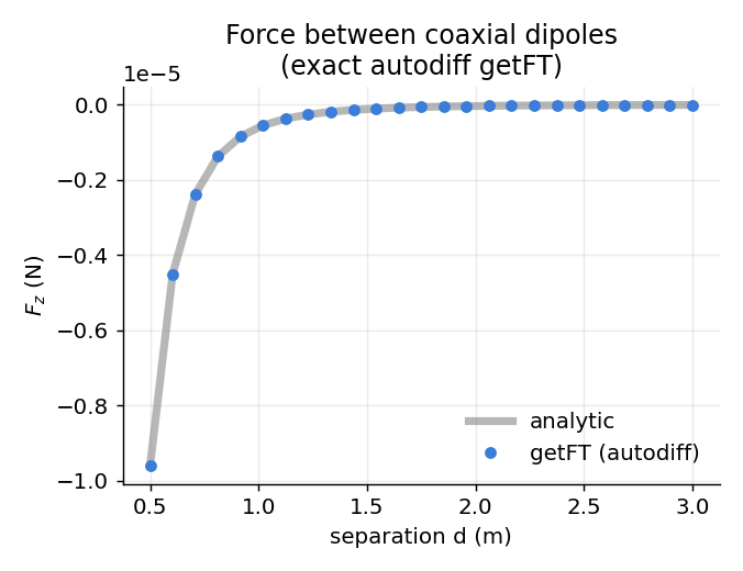
Force versus distance
Sweeping the target position and plotting |F| against separation produces the characteristic
decay below. jax.vmap evaluates the whole sweep in one vectorized call.
import jax
import jax.numpy as jnp
import magpylib_jax as mpj

jax.config.update("jax_enable_x64", True)

coil = mpj.current.Circle(current=200.0, diameter=0.02)


def force_at(z):
    magnet = mpj.magnet.Cuboid(
        dimension=(0.005, 0.005, 0.005),
        polarization=(0.0, 0.0, 1.2),
        position=(0.0, 0.0, z),
    )
    F, _ = mpj.getFT(coil, magnet)
    return jnp.linalg.norm(F)

zs = jnp.linspace(0.008, 0.05, 60)
F_mag = jax.vmap(force_at)(zs)
See also
Optimization examples — differentiable inverse-design loops for the field itself.
Equation Models — closed-form field models and the force/torque derivation.
Visualization with show() — inspect source and target geometry in 3D.