Visualization with show()
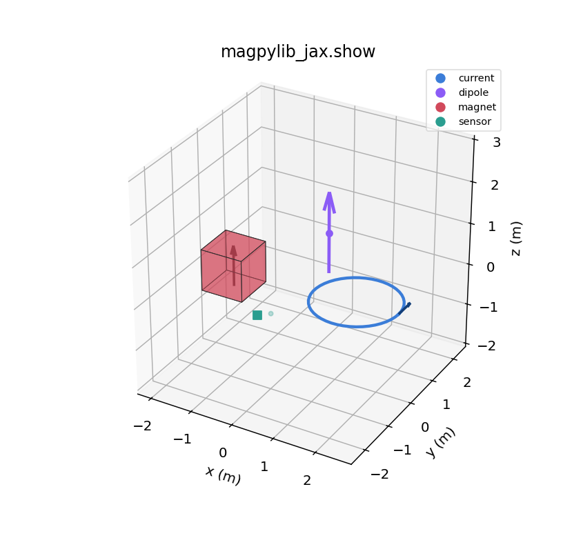
magpylib_jax ships a lightweight matplotlib 3D renderer for inspecting source, sensor, and
collection geometry. It is available both as a free function, mpj.show(...), and as a .show()
method on every object.
Note
The renderer is for geometry inspection, not field visualization. Use the field API
(getB/getH) together with your own plotting code for field maps.
Basic usage
Pass any number of sources, sensors, or collections to mpj.show:
import magpylib_jax as mpj

coil = mpj.current.Circle(current=1.2, diameter=0.6)
magnet = mpj.magnet.Cuboid(
    dimension=(0.4, 0.3, 0.2),
    polarization=(0.0, 0.0, 0.7),
    position=(0.0, 0.0, 0.5),
)
sensor = mpj.Sensor(pixel=[(0.0, 0.0, 0.2), (0.0, 0.1, 0.2)])

mpj.show(coil, magnet, sensor)
Every object also carries a .show() method that renders it on its own:
magnet.show()
A Collection renders all of its children in one scene:
system = mpj.Collection(coil, magnet)
system.show()
Composing with your own axes
Pass an existing 3D axes through ax= to draw into a subplot you control — useful for
side-by-side layouts or for overlaying show() output with other matplotlib content:
import matplotlib.pyplot as plt

fig = plt.figure(figsize=(11, 5))
ax_left = fig.add_subplot(1, 2, 1, projection="3d")
ax_right = fig.add_subplot(1, 2, 2, projection="3d")

mpj.show(magnet, ax=ax_left)
mpj.show(coil, sensor, ax=ax_right)
fig.tight_layout()
When you supply ax, show() draws into it and does not create or display a new figure.
Returning the figure
Set return_fig=True to get the matplotlib.figure.Figure back instead of showing it. This is the
right choice for headless rendering, saving to disk, or tests, and it never calls plt.show():
fig = mpj.show(coil, magnet, sensor, return_fig=True)
fig.savefig("system.png", dpi=150)
Titles and styling
A title can be set through either title= or a style mapping:
mpj.show(coil, magnet, title="Coil and magnet")
mpj.show(coil, magnet, style={"title": "Coil and magnet"})
Objects can also carry a style_label, which is used to annotate the object marker in the scene.
What each object renders
The renderer color-codes objects by physical category (magnets red, currents blue, dipoles purple, sensors teal, custom sources grey) and draws a legend for the categories present.
- Magnet sources (red)
Cuboid,Cylinder,CylinderSegment, andSphererender as their solid bodies;Tetrahedron,TriangularMesh, andTrianglerender as their oriented faces.- Current sources (blue)
CircleandPolylinerender as their conductor path;TriangleStripandTriangleSheetrender as their triangle faces.- Dipole sources (purple)
Dipolerenders as a moment arrow through its position.- Sensors (teal)
Sensorrenders as a square marker with its pixel points and local axis arrows.- Custom sources (grey)
CustomSourcerenders as a labeled position marker.
Multi-point motion paths are drawn as a dashed trailing line, and the body itself is drawn at the final pose on the path.
Backends
Only the matplotlib backend is provided. Requesting another backend raises a ValueError:
mpj.show(magnet, backend="matplotlib") # the only supported value
Interactive backends such as plotly and pyvista, which upstream Magpylib offers, are not
(yet) implemented here. matplotlib must be installed; it is included in the docs and test
extras.
See also
Object API examples — building the sources and collections shown here.
Force and torque (getFT) — inspect target geometry alongside force computations.